Naive Bayes authorship classification with Facebook Messenger data ::

1.1 Introduction

Many of us have easy access to an incredibly rich, personalised textual dataset.

Facebook

I have had a Facebook profile since my early high school years. I have access to hundreds of Facebook Messenger conversations to which I have contributed for over a decade. In other words, I have access to an enormous amount of textual data, comprising not only all the written words that I’ve sent over Messenger but also the words that my friends have sent to me.

At the time of writing, Facebook does not delete messages once they are past a certain expiry date, unlike some other messaging apps (e.g., Microsoft Teams). Our pools of conversations can be uncovered easily, years after each data droplet was formed with our keyboards. Sure, it may take some scrolling, but a couple of search terms can very easily bring up the deepest depths of our conversations from some of our most vulnerable and juvenile moments on this Earth.

The existence of this bizarre, superfluous word archive at my fingertips sparked a new project idea. Sure, in a way, it’s awful that so many of the terrible, terrible takes of our pasts are still sitting out there on Facebook servers, perpetually on standby to be retrieved by whoever has the access, the interest, and a link to the conversation in question. So, why wouldn’t I take advantage of this uneasy situation and make a fun learning project out of it?

My thoughts culminated into one focused project idea: an authorship classifier. One that is trained on Facebook Messenger data.

1.2. Background: Authorship classification

Classification is a massive part of what we do with our human intelligence. We sort paper mail by postal address, identify people we know on the street by recognising their faces, judge whether or not we thought that the film we just watched was actually good, or just weird in a bad way…

In a classification process, we gather data about a certain ‘thing’ (which could come from multiple sources) and assign a particular category to it.

As a useful tool, many methods of machine intelligence have been developed for classification tasks. In the realm of natural language processing, text categorisation methods have been developed to assign a label or category to an entire text or document. Some tasks that come to mind include:

sentiment analysis - e.g., analysing whether a review of a book is positive or negative)
spam detection - filtering out emails that have indicators of being spam)
language identification – identifying the language in which a text is written

The method of authorship classification (also referred to as authorship attribution), takes a textual document, processes it, and then categorises it as being written by a particular individual, or author. Such a task has useful applications in the real world – for example, plagiarism detection in the education system, or resolving uncertain authorship of documents in forensic studies.

As is very often the case in computing disciplines, there isn’t just one way to build a tool that does authorship classification. Over the last couple of decades, research scientists and industry developers have studied and applied a range of methodologies for the task. The methods explored can be categorised under a few umbrellas, some of which include:

similarity-based models, which measure how similar an input text is to the textual data collected for that author, e.g., how many words in the text being classified overlap with the words collected for an author in their training data
probabilistic models, which calculate the probability of each author creating the input string of words
vector-space models – processing the text being classified by transforming the words into a vector representation

For this project, I chose Naive Bayes Classification as the model behind my authorship classifier. I thought that this would be a good model to start with for learning purposes, as it is a simple model that can be used to classify many different types of data, is more straightforward to implement, and tends to have solid performance. A great learning source that I used to familiarise myself with the method was the ‘Naive Bayes and Sentiment Classification’ chapter in Jurasfky and Martin’s Speech and Language Processing book.

1.3. Naive Bayes Classification: an explanation

In the context of authorship attribution, the Naive Bayes classification method applies Bayesian inference to calculate the most likely author to have written a given document.

Bayesian inference, which originates from the 18th-century work of Thomas Bayes, works with conditional probabilities. Bayes’ theorem is stated in the mathematical equation:

Naive Bayes

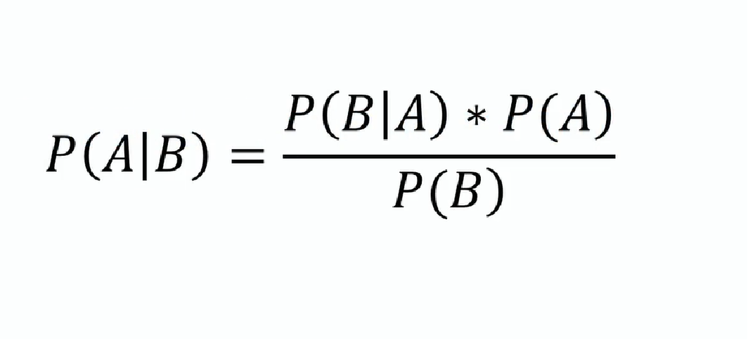
In the right-hand side of the equation above, we’ve got three variables:

P(B|A) – a conditional probability, that is, the probability of an event B occurring given event A. This is also called the likelihood of event A given a fixed B.
P(A) – the probability of event A, without P(B) in the picture. This is also called the prior probability.
P(B) – the probability of event B, without P(A) in the picture. This is also called the marginal probability.

The above explanation is abstract, so let’s see how it would apply in our context of authorship classification.

P(A|B) becomes P(author|document) - that is, the probability of an author being classified given a document being processed.
P(B|A) becomes P(document|author) - that is, the probability of a document being written given the existence of an author.
P(A) – the prior probability of an author. In our context, this would represent the proportion of an author’s writing existing in our training data, out of all the other authors’ writings in the training data.
P(B) – the marginal probability of the document data, in relation to other document data. This variable is actually irrelevant for our classification task – the task is focusing on one document at a time with each run of the classifier. Other than the input text, no other data are are being considered for authorship classification during each run. So, we are conveniently going to drop this variable from our equation.

After dropping P(B) from our equation, it reduces to:

P(author|document) = P(document|author) * P(author)

Naive Bayes

You might be thinking: how are we fitting that entire ‘document’ into our equation here? Wouldn’t we have to break down the document into parts, analysing the different linguistic features inside the document and seeing which features correspond to which author?

And that would be a good question!

The way we are defining our ‘document’ for this task is by simply seeing it as a “bag of words”. The classifier is going to process the entire thing word-by-word and see what vocabulary is used in that document. Then, it will compare that vocabulary with the words that are used by each author in their training data.

The concept of seeing the document as a “bag of words” means that we will consider the presence of each vocabulary item as an individual entity, without considering its co-occurrence with any other vocabulary item or linguistic feature. We know that in linguistic reality, words very much co-occur with one other in very systematic ways, and they don’t often just appear randomly by chance. However, the ‘Naïve’ part of this classification model assumes that each feature (i.e., word) used by an author is an independent event in itself. By assuming independence, you are then able to easily calculate the overall probability of the document occurring by multiplying the chance that an author would use each one of those vocabulary items.

So, we could rewrite our previous equation to be:

P(author|word1, word2, word3, …, wordn) = P(word1 * word2 * word3 * …wordn | author) * P(author)

Otherwise stated, we are multiplying the likelihoods of each vocabulary item appearing in the text, regardless of their position within the document. Overall, it’s a very simple way of gauging the probability of an author having written a text – we don’t pay attention to any other linguistic feature other than the presence of certain words.

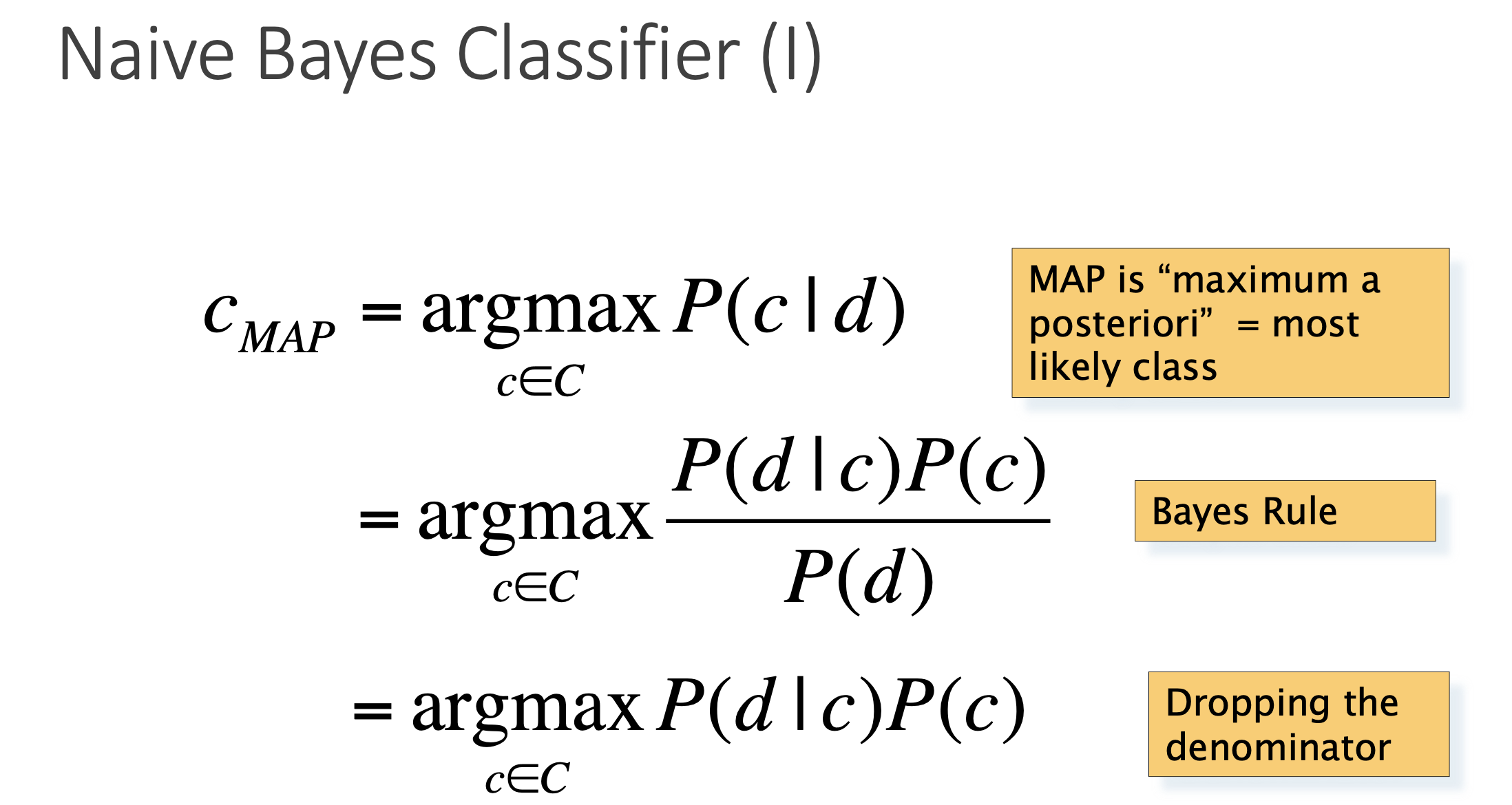
Upon execution, the classifier runs this Bayesian calculation for each author in the candidate set. It returns the author with the maximum overall posterior probability (i.e., P(author | document) out of all the runs for the authors. This is the output – a classified author!

In a mathematical formula, the concept of returning an author with the maximum posterior probability can be written as such:

In our applied context, it would look a bit more like this:

Run 1: P(‘Joan’|word1, word2, word3, …, wordn) = P(word1 * word2 * word3 * …wordn | ‘Joan’) * P(‘Joan’) = 0.125

Run 2: P(‘Don’|word1, word2, word3, …, wordn) = P(word1 * word2 * word3 * …wordn | ‘Don’) * P(‘Don’) = 0.223

Run 3: P(‘Roger’|word1, word2, word3, …, wordn) = P(word1 * word2 * word3 * …wordn | ‘Roger’) * P(‘Roger’) = 0.08

In the runs above, Run 2 (Don) has the highest posterior probability returned (0.223), so Don would be returned as our classified author.

For the problem of text classification, it’s very useful to convert the conditional probabilities into log form. The reason for this is that the probabilities of each word being used is often very small (since there are so many words out there) and multiplying each one of them together creates a very, very small number with lots of zeroes. So many zeroes in fact, then when you scale that calculation up, there is a risk of arithmetic underflow! So, log form solves this issue by converting that very small number into a more palatable negative integer. Note that when you work with log numbers, you add them together instead of multiplying them:

P(‘Joan’|word1, word2, word3, …, wordn) = log(P(word1| ‘Joan’) + log(P(word2| ‘Joan’) + log(P(word3| ‘Joan’)), …, + log(P(wordn| ‘Joan’)) + log(P(‘Joan’)).

2. Implementing the Classifier

To implement a Naïve Bayes authorship classifier, there are a number of variables to keep in mind.

The different variables (i.e., parts) of the classifier can be summarised in the following list:

A set of authors as ‘candidates’ for classification, e.g. [Joan, Don, Roger]
Some training data, that is, the balanced set of textual data made of up real text written by each of the candidate authors, to train your classifier on
Some test data, that is, a set of textual data collected from the candidate authors that helps you measure how well your classifier is performing after you have trained it on the training data. Here is a rule of thumb that I have seen with allocating training and test data - 80% of your collected author data can be training data, and the remaining 20% can be test data.
A training function, that is, a function that trains the classifier on training data
A applied function, that is, a function that applies the classifier to test data

In my case, I placed the training data in one folder, the test data in another folder, and both the training and testing function in the same Python script.

2.1. Collecting the author candidate data from Facebook Messenger

The very first thing I considered before collecting my friends’ data, for a publicly shared project like this, was to get the consent of my selected friends first to use their data in this way.

After all, my friends originally expressed their thoughts with me on Facebook Messenger under the presumption that it would stay within the bounds of our private conversation. So, I would like to reiterate that if you decide to use someone’s personal data for a publicly-shared project – be sure to explain to them that you are planning to collect their private data for a personal project, and explain clearly what you would be doing with their data after they give you their permission. This gives them a chance to say yes or no to what you are doing with their data. If you feel like you can’t ask your friend’s permission – then don’t use their data. Consent is key.

I managed to get the permission of two of my close friends to extract our Facebook Messenger conversations and create ‘textual data pools’ for both of them. I also included my own data in this project.

So, as it stands, there are three authors for my classifier:

Amelia
Lewis
Gina (me)

To scrape the Facebook Messenger conversation data, I used the fbtxtscaper tool. This neat script allows you to log into your Facebook account programmatically, extract an entire conversation history between you and your friend, and store that data in a CSV file. Each row of this CSV file contains messages sent at a certain time by each author.

To work with that CSV file and covert it into textual data ‘pools’ for each author, I wrote some code that would take the CSV file, extract words from each line that is labelled with a certain author (using the csv module) , and put those words in a text file.

Here is an example of that code applied to author ‘Lewis’:

import csv

csv_data = []

# read CSV file
with open('fb_text_lewis_gina.csv', newline='') as csvfile:
    csv_reader = csv.reader(csvfile)
    for line in csv_reader:
        csv_data.append(line)

# add contents of CSV file to lewis_data.txt
for line in csv_data:
    if line[1] == 'Lewis Ives':
        with open('lewis_data.txt', 'a') as f:
            f.write(line[2] + ' ')
f.close()

The result is a text file that contains a pool of textual data for that particular author ([author]_data.txt’).

After running that extraction for each of the candidate authors, I had some big, heavy text documents to work with.

My friend Amelia and I had heaps of words in our data sets, which reflects on the fact that we’ve been friends for several years and we have regularly used Facebook to message each other for several years.

On the other hand, my friend Lewis and I have only been friends for just over a year, and we don’t use Facebook Messenger as often to interact with each other, other than mainly to coordinate real-life plans together.

This created an imbalance in the data sets – Lewis’ training dataset only had 10,000 words, whereas Amelia and I had close to 100,000 each. I wanted the data sets for each other to be of equal length, in order to ensure that the training data were balanced and to reduce the chances of the classifier being biased towards a particular author candidate. So, I cut down my and Amelia’s data to 10,000 each, so that the priors for each candidate author – P(author) - could accurately be one third (1/3) each.

In projects that deal with natural language data, it is also important to remember the pre-processing step of tokenising the textual data. Tokenising textual data allows the data set to be processed by the classifier as a document of words and word parts, instead of one giant string of random characters.

I used the below code as a function to tokenise the training data documents of each author candidate:

import nltk
from nltk.tokenize import word_tokenize
from nltk.tokenize import sent_tokenize

def extract_words(file):
    dataset =[]
    with open(file, 'r') as fh:
        dataset = fh.read()
        fh.close()
    word_dataset = word_tokenize(dataset)
    return word_dataset

I applied this function to each training and test document that I was working with, so that I had a set of variables containing tokenised word data to refer to in my Naive Bayes Classifier script:

# training datasets
amelia_document = extract_words('amelia_training_data.txt')
gina_document = extract_words('gina_training_data.txt')
lewis_document = extract_words('./training_data/lewis_training_data.txt')

# test datasets
amelia_test_doc = extract_words('./test_data/amelia_test_document.txt')
gina_test_doc = extract_words('./test_data/gina_test_document.txt')
lewis_test_doc = extract_words('./test_data/lewis_test_document.txt')

Overall, the steps for data collection for this authorship classifier can be summarised as follows:

Use a web scraping tool that can access and extract entire Facebook Messenger conversations,
Separate the conversational data into ‘pools’ for each candidate author,
Make sure that the training data is balanced (in number of words) between the candidate authors,
Make sure that your training data is tokenised, so that you are working with real words as data, not just strings of characters.

2.2. Feature selection

Before we get started on implementing the classifier itself, I’ll drop a couple of notes on feature selection.

The Naive Bayes classification method considers features of the data in order to make its class prediction. In our application of the method to text author classification, the classifier considers the presence of vocabulary items within the textual data as features.

A major problem in the realm of text classification is in the high dimensionality of the feature space in the domain of textual data. We can attribute the problem to the fact that in human language, many unique words are used to string together paragraphs of expression. In our classifier’s training data, our candidate authors use thousands of unique vocabulary items. Since we are keeping tabs on the conditional probabilities of vocabulary items, this means that our domain has thousands of potential features to work with. Overall, when a classifier has a very high number of features to consider when calculating conditional probabilities, its performance - in terms of speed and even accuracy - can be lowered considerably.

A way of accounting for high dimensionality is to perform feature selection. This process prunes the number of features for the classifier in order to reduce the feature space. When pruning the feature space, we have to make decisions on which features would be most relevant for the classifier to consider.

I narrowed down the set of words in the feature space (i.e. the vocabulary of the classifier)

# extract 50 most common words from each author's training data

amelia_freq_dist = [i[0] for i in FreqDist(amelia_document).most_common(50)]
gina_freq_dist = [i[0] for i in FreqDist(gina_document).most_common(50)]
lewis_freq_dist = [i[0] for i in FreqDist(lewis_document).most_common(50)]

# merge vocabulary into set

vocabulary = set(amelia_freq_dist + gina_freq_dist + lewis_freq_dist)

You can see that I’ve taken the 50 most common words for each author and placed that in a merged set ‘vocabulary’ as the feature space.

The idea behind this was that I wanted the feature space to contain words that each author is most likely to say, to encapsulate the vocabulary items that are characteristic of each author.

I did try another method of feature extraction. At one point, I made the feature space to be the merged set of ‘unique vocabulary’ of each author, that is, any vocabulary item in the training data that was written by one author, but not by the other two. The problem with this feature space was that the frequencies of these unique vocabulary items tended to be incredibly low. Often when running the classifier on the test document, the document itself did not contain enough of these unique vocabulary items, to the point that the classifier simply could not get enough information from the text to make a good classification.

So, I went back to making the feature space as the top 50 frequency words for each author – even though a lot of these words would overlap, there would be enough of a sample size for the feature space to contain some less frequent (but distinct) vocabulary items of each author.

Overall, making decisions on the feature space of the classifier can have a big impact on its accuracy and performance.

2.3. Implementing the Naive Bayes Classifier

As a place to start, I referred to the pseudocode written out in Jurasfky and Martin’s chapter in order to get an idea of how I would start to implement the classifier in Python.

As mentioned above, we have two main parts to the classification script:

the training function
the testing function

This is how the training function was implemented in my Python script:

def train_naive_bayes(authors, vocabulary):

    all_words = amelia_document + gina_document + lewis_document
        n_documents = len(all_words)
    authorship = {“Amelia”: amelia_document, “Gina”: gina_document, “Lewis”: lewis_document}
    log_priors = {}
    log_likelihoods = {}
    n_authored_data = {}

    for author in authors:
        log_priors[author] = 1/(len(authors))
        n_authored_data[author] = len(authorship[author])
        log_likelihoods[author] = {}
        for unique_word in vocabulary:
            counter = authorship[author].count(unique_word)
            log_likelihoods[author][unique_word] = math.log(counter+1)/(n_authored_data[author]+1*(all_words.count(unique_word)+1/n_documents+1))

    return log_priors, log_likelihoods

Let’s break down the training function into its component steps:

Load the candidate author set and feature space (i.e. vocabulary) into the train_naive_bayes function
```
 def train_naive_bayes(authors, vocabulary)
```
Keep track of the content and length of the entire training dataset. Initialise the relation between the candidate author label and their training document, by creating a dictionary ‘authorship’ that links one with the other:
```
 all_words = amelia_document + gina_document + lewis_document
 n_documents = len(all_words)
 authorship = {“Amelia”: amelia_document, “Gina”: gina_document, “Lewis”: lewis_document}
```
Initialise the dictionaries that record the log priors, log likelihoods and the length of each author’s training document:
```
 log_priors = {}
 log_likelihoods = {}
 n_authored_data = {}
```
Fill in the above variables by cycling through the candidate author set and creating dictionaries that track the relevant values for each author. For the log_likelihoods variable, I created a nested dictionary, since the conditional probabilities of several vocabulary items will need to be tracked for each author (not just one item):
```
 for author in authors:
     log_priors[author] = 1/(len(authors))
     n_authored_data[author] = len(authorship[author])
     log_likelihoods[author] = {}
```
Now time for the actual calculation of the conditional probabilities. The script cycles through the input vocabulary (feature space), and counts how many times that vocabulary item appears in each author’s training document.
```
 for unique_item in vocabulary:
     counter = authorship[author].count(unique_word)
```

For that vocabulary item, I then took the count of how many times it appears in that training document and added 1 to it (see LaPlace smoothing), divided that value by the length of the training document (plus 1), and multiplied that value by the number of times that the vocabulary item appears in all training documents (plus 1), out of all the words that appear in all the training documents (plus 1). Then, convert that whole calculation into its log value, using the math module in Python.

log_likelihoods[author][unique_word]=
math.log((counter+1)/(n_authored_data[author]+1*(all_words.count(unique_word)+1/n_documents+1)))

Return the log priors and log likelihoods. The output of this function can then be assigned as global variables for the rest of the script to work with.
```
 return log_priors, log_likelihoods
 log_priors, log_likelihoods = train_naive_bayes(authors, vocabulary)
```

2.4. Testing

Now that I had the training function implemented, it’s time to actually apply it to some real test data.

def test_naive_bayes(testdoc, logpriors, loglikelihoods, authors, vocabulary):
    sums = {}

    # process test doc
    for author in authors:
        sums[author] = logpriors[author]
        for word in testdoc:
            if word in vocabulary:
                # add author's conditional likelihood of vocab item to sums value
                sums[author] += loglikelihoods[author][word]

    # return author with maximum posterior probability
    for author in sums:
        if sums[author] == max(sums.values()):
            return "Author classified: " + author

Again, let’s break the test_naive_bayes function into its steps:

Load the test document, log priors and log likelihoods (from the training function), author candidate set and vocabulary into the test function:
```
def test_naive_bayes(testdoc, logpriors, loglikelihoods, authors, vocabulary):
```
Create a dictionary called “sums” that will keep track of each author, as well as a counter for how often a vocabulary item appears in the test data. Initialise the value this dictionary as the log prior value for each author (calculated in the training function):
```
sums = {}
for author in authors:
    sums[author] = logpriors[author]
```
Cycle through every token in the test document. If that token also appears in the vocabulary list, then add the author’s log likelihood of that word (calculated in the training function) to the author’s value in the “sums” dictionary.
```
 for word in testdoc:
     if word in vocabulary:
         sums[author] += loglikelihoods[author][word]
```

The more words in the test document that appear in the vocabulary, and the more that vocabulary appears in the training data of an author, the higher the “sums” value will be for that author – that is, they are more likely to be the author for that test document (based on Naive Bayesian inference):

To explain this calculation a bit further – overall, the classifier is trying to link the frequency of vocabulary items appearing in the test document with the frequency of those items appearing in each author’s training document. For each vocabulary item, the testing function sees how often it appears as a word in the test document. Each time that item is detected in the test document, the author’s “sums” value increments by the conditional likelihood value of that vocabulary item in the author’s training data (loglikelihoods[author][word]).

Take the example of the vocabulary item ‘like’. In my section of the log likelihoods dictionary (author: ‘Gina’), the log probability for this item is -1.2645269104588241. In the the classifier’s test run that calculates my likelihood of being an author candidate, every instance of the word ‘like’ appearing in the test document would increment my “sums” value by -1.2645269104588241 each time.

The word ‘like’ appears 4 times in training document:

sums[‘Gina’] = -0.47712125472 (log prior) + 
(-1.2645269104588241 ) + 
(-1.2645269104588241) + 
(-1.2645269104588241 + 
(-1.2645269104588241)`

> Summed value: -5.53522889656

Let’s take that same example word ‘like’, and let’s imagine that the log probability was a lower value at -9.134236087786782. Maybe, it would be the result of the word ‘like’ appearing much less in the training document of the author ‘Amelia’:

sums[‘Amelia’] = -0.47712125472 (log prior) + 
(-9.134236087786782) + 
(-9.134236087786782) + 
(-9.134236087786782) + 
(-9.134236087786782)

> Summed value: -37.0140656059

The word ‘like’ still appears 4 times in this classifier run, since the test document is the same. However, the word contributes way less to the “sums” value of the author Amelia, since her conditional likelihood of this word in her dictionary is much lower.

If the test document contains a high frequency of vocabulary items, and an author’s training data also contains a high frequency of those items, the “sums” value of that author is going to be higher than the others. According to the classifier, they are a more likely candidate to have authored that document, since the vocabulary items have a high rate of co-occurring in both the test document and the author’s training document. On the other hand, if you have a high number of vocabulary items appearing in the test document, but hardly any them appear in the training data of an author, then that particular author’s “sums” value will be lower, making them a less likely candidate to have authored that document.

The last step of the code cycles through the authors in the “sums” dictionary. It returns the author with the highest “sums” value – this is the most likely candidate author, according to the classifier:

 for author in sums:
     if sums[author] == max(sums.values()):
        return "Author classified: " + author

In other words, we have run the test classifier on all the different authors, calculated the “sums” for each one, and will return the author that had the highest value in their “sums” calculation.

To make the results clearer to me, I also wrote a small function that prints out the results neatly to my console:

 def print_out_test(doc_string, real_author):
 print("Real author: " + real_author + " --> " + test_naive_bayes(doc_string, log_priors, log_likelihoods, authors, vocabulary))
 return 
 
 print_out_test(text_file.txt, 'Author')
 > “Real author: 'Author' --> Author classified: 'Author'”

Overall, the implementation of the training and testing functions did not take up much code at all. I managed to fit it all in to about 30 lines – a testament to the simplicity of the Naive Bayes classification method.

3. Results

3.1. The output

I had a bit of trial-and-error in applying this classifier to the test documents using different methods of feature extraction. My goal was to get it to classify each test document (n words =10,000 each) of the author as the correct one. After much fiddling around (and fixing bugs along the way), I finally got it classifying the correct authors:

print_out_test(amelia_test_doc, "Amelia")
print_out_test(lewis_test_doc, "Lewis")
print_out_test(gina_test_doc, "Gina")

>> “Real author: Amelia --> Author classified: Amelia”
>> “Real author: Lewis --> Author classified: Lewis”
>> “Real author: Gina --> Author classified: Gina”

Also, a fun thing to do is to put in random strings as input, and get the classifier to guess which one of your friends is most likely to write something like that:

(1) print_out_test(“heyo, :^)”, “N/A”)

>> “Real author: N/A --> Author classified: Lewis”

(2) print_out_test(“I’m really hungry, really want some choccie…sad”, “N/A”)

>> “Real author: N/A --> Author classified: Gina”

I want to emphasise that the results were by no means perfect – even though the whole test documents were correctly classified, failures did happen when I took subsets of training data to test the classifier.

(3) print_out_test(“mmm I’ll try to get there like 9 maybe? Ye that is ok! I wanna leave early cos it’s a long drive Cool cool, I’ll message you tomorrow morning I think I’ll be more like 9:30 but I’ll msg you”, “Amelia”)

>> “Real author: Amelia --> Author classified: Gina”

3.2. Insights

One thing I noticed was that the classifier was very good at correctly classifying one of the authors (Lewis) but found it harder to distinguish between the other two authors (Amelia and Gina).

I think that the classifier’s difficulty in distinguishing between Amelia’s and Gina’s (my) data may have had to do with the context in which their training data were collected. The source of these two authors’ training data was the same – their words were extracted from the same conversation between each other. Lewis’ training data, on the other hand, were extracted from a conversation with me, but my data were not extracted from this same source. When I look at my and Amelia’s conversation thread with the naked eye, I can see that we often mirror each other with our language choices, probably due to our close camaraderie and inside jokes. In a way, the collection of our training data would not be so much a representation of our word choices across all domains, but rather a representation of our word choices in relation to when we interact with each other.

So, there’s a sort of asymmetry going on in the domains across the training data. Amelia’s training data is based on Gina-Amelia conversations (but not Lewis-Amelia); Lewis’ training data is based on Lewis-Gina conversations (but not Lewis-Amelia), but Gina’s training data is based on Gina-Amelia conversations (but not Lewis-Gina). I think it would be interesting to see how this classifier would perform if the domain gaps mentioned here were filled.

Or, you could have another kind of textual data – capturing monologues of each author so that you have data that is not expressed in relation to another person, like academic essays. However, you would probably have to test a classifier that is trained on this kind of data with a test document that is also a sort of monologue.

4. Conclusion

I found the implementation of the Naive Bayes classification method with Python relatively simple to do. I think it would be cool to experiment with this classification method with other types of features (e.g., character trigrams), other types of training data, and more authors.

Overall, this endeavour was a solid intro to classification methods, and it taught me the basics of Bayesian inference from an applied point of view. I could write the entire classifier script in less than 75 lines. I think it performed well given that it considered just one type of linguistic feature, was trained on a relatively low amount of data, and had a very simple code implementation. It’s nice to have in the toolkit!